Liquid Simulation with Tetrahedral Meshes
 |
M.S. Comprehensive Examination Project |
Project Overview
The purpose of this project is to demonstrate an understanding of numerous concepts in computer graphics and physics-based animation through a challenging area of research – liquid simulation. Animating fluids has been a particularly difficult problem in computer graphics as the physical laws that govern fluid dynamics are complex and modeling them realistically is computationally expensive. We are interested in simulating free-surface fluids, where a free-surface is the boundary between two fluids – in our case, liquid and air. This is more challenging than fluids with no free surfaces - such as gas flowing through a static simulation domain - since the free-surface must be maintained explicitly and usually in high detail.
This project is heavily based on the work of Chentanez et al. [CFLOS07], but customizations were made to accommodate a simulation mesh of lower resolution to that of the authors’, due to performance issues. This page will highlight these modifications while presenting the overall methodology for the liquid simulation, as obtained from many different sources.
Different models exist for animating fluids, and among the most popular are regular hexahedral grids or mesh-less collections of points. However, [CFLOS07] advocate the use of un-structured tetrahedral meshes (a tetrahedron is like a pyramid, except with a triangular base) since they more easily conform to complex boundaries and tetrahedra can vary in size to focus computation near the surface where more detail is required.
This implementation is written in C++ and uses OpenGL for the graphical test display. It uses semi-Lagrangian contouring for surface tracking, provided by Bargteil et al. [BGOS06] as Open Source code. It also uses the CLAPACK library written in C for solving small linear systems. All animations were rendered using PIXIE, an Open Source renderer (uses the RenderMan interface).
Movie Quick Links (more details below)
References
-
[LS07] Labelle, F., Shewchuk, J.: Isosurface stufffing: fast tetrahedral meshes with good dihedral angles. ACM Transactions on Graphics 26, 3 (2007).
-
[Sta99] Stam, J.: Stable fluids. In Computer Graphics (SIGGRAPH ’99 Proceedings) (Aug. 1999), 121-128.
|
Governing Equations |
|
We are interested in simulating Newtonian fluids (i.e. flows like water) that are governed by the Euler equations for inviscid (non-viscous) fluids, |
|
|
|
(1) |
|
where u is the
fluid velocity field, p is the pressure field, t is time,
We assume the fluid is incompressible and must conserve its total volume. We apply the constraint |
|
|
|
(2) |
|
specifying that the divergence of the velocities across the fluid must equal zero. In other words, for an infinitesimally small region of the fluid, all velocities that flow into the region must equal the amount of velocities that flow outward. |
|
|
Overview of Simulation |
|
It is customary to integrate each term of Equation (1) into separate operations: |
|
|
|
(3) |
|
|
(4) |
|
|
(5) |
|
|
(6) |
|
where
|
|
|
Time Step |
|
At the beginning of each simulation time step t,
we have a surface contour St (in the form of a high resolution
triangulation) for tracking the surface and a volumetric tetrahedral mesh Mt
which stores the velocity field
|
|
Semi-Lagrangian Contouring |
|
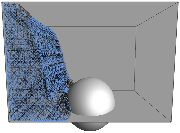
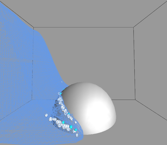
We track the surface of the liquid using semi-Lagrangian contouring (SLC) [BGOS06]. The goal is to compute a new liquid boundary from a previous time step’s liquid boundary and a velocity field defined over the previous tetrahedral mesh. We use the semi-Lagrangian advection method to determine this new boundary. SLC employs an implicit representation as a signed distance function (using an octree structure) with a zero level set that defines the surface. This implicit representation can easily handle large topological deformations whereas an explicit representation would quickly encounter tangling and cross-intersections of the surface. SLC also constructs an explicit representation (from the implicit representation) as a high resolution triangulation of the surface using Marching Cubes, shown to the right. This explicit representation supports the exact calculation of signed distances near the surface, while approximating (quickly) far distances from the surface by interpolating over the octree. The resulting signed distance function of the new surface is conveniently compatible with our mesh generator, which takes this function as input. |
|
|
Mesh Generation |
|
We build a tetrahedral mesh that approximates a given volume using the Isosurface Stuffing Algorithm [LS07], shown to the right. This work was completed as a project from a previous course, but various optimizations and additions were necessary for its use in simulation. To use the mesh in simulation, we store additional values in the tetrahedra and triangular faces. We store a scalar pressure value at the center of each tetrahedron. At the center of each face, we store the scalar component of velocity normal to the face. It might seem more reasonable to store full velocity vectors in the center of tetrahedra, but this storage scheme aids an efficient discretization during the pressure solving stage without sacrificing the ability to recover these full velocity vectors exactly from face normal velocity components. |
|
|
Semi-Lagrangian Advection |
|
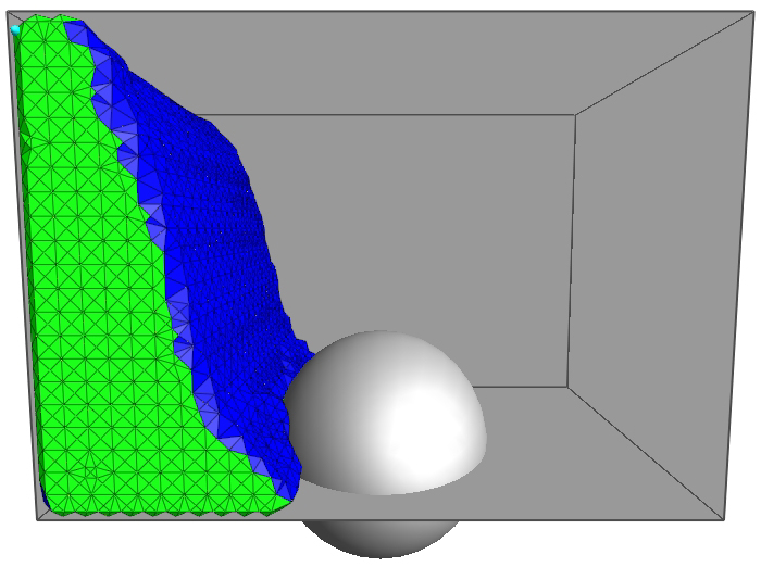
Advection is transport in a fluid, describing the behavior of how, for example, material/scalar concentrations (e.g. dyes, heat, pollutants, etc.) flow through a fluid given a velocity field. We turn to the popular semi-Lagrangian advection method to model this, originally pioneered by Stam [Sta99] and generalized by Feldman et al. [FOKG05] to account for mesh deformations between time steps. We apply this technique for advecting both the surface contour and mesh velocities using the previous time step’s velocity field, shown to the right. The idea is to start from a new location in the current time step, use the velocity at the new location from the previous time step to trace a path backwards to an old location, then assign the velocity at this old location to the new location. The intuition behind this method is to determine which velocity flowed to the current location from the previous time step. In our case, we trace paths back from each face center in the new mesh and assign them velocities from the old mesh. However, this is not a straightforward process as the mesh topology changes between time steps and tracing paths back usually falls between known velocities. To deal with this, we must use interpolated or extrapolated velocities at arbitrary locations in the old mesh. |
|
|
Velocity Interpolation |
|
We begin the advection process by computing velocities at tetrahedron centers from their four face normal velocity components. We use the method described in Klingner et al. [KFCO06] by solving the small, over-determined linear system of equations in the least squares sense |
|
|
|
(7) |
|
where To interpolate a velocity at an arbitrary location in the mesh, we use the generalized barycentric interpolation method as described in [KFCO06]. We locate the closest vertex in the mesh to this location and determine the Voronoi cell associated with this vertex (i.e. the Voronoi cell consisting of all tetrahedra that share this vertex). We use the following equation to compute an unnormalized weight for each tetrahedron t in the Voronoi cell: |
|
|
|
(8) |
|
where |
|
|
|
(9) |
|
where |
|

|
Velocity Extrapolation |
|
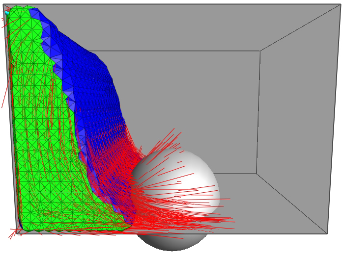
Occasionally a path is traced outside of the mesh which requires us to extrapolate velocities to the octree (i.e. extend the boundary of the velocity field), shown to the right. We use the method employed in Losasso et al. [LGF04] and Enright et al. [EMF02], but described in Adalsteinsson et al. [AS99]. We first determine the octree vertices that lie outside of the mesh. The authors originally include only a band of vertices within a distance threshold from the mesh, but in practice it is not computationally expensive to include all octree vertices when using a lower resolution mesh. We then sort the vertices by their signed distance values from closest to farthest from the surface. By iterating over vertices in this order, we ensure that we are extrapolating with the most accurate velocity information available at each vertex. For each vertex, we compute the velocity according to the equation |
|
|
|
(10) |
|
where
Once velocities are extrapolated to octree vertices, we can determine the velocity at an arbitrary point by trilinear interpolation over the eight corner velocities of the containing octant. |
|

|
Tracing Back Velocities |
|
[CFLOS07] observed that using a smoothed version of the velocity field for tracing paths does not produce objectionable artifacts. They first compute velocities at all mesh vertices by generalized barycentric interpolation then use standard barycentric interpolation (within a single containing tetrahedron) to more efficiently trace paths. While this may be true for high resolution simulations, at lower resolutions the artifacts are more noticeable and the fluid flow appears less accurate. Therefore, we use generalized barycentric interpolation for tracing back paths (albeit at a computational cost). Once a path has been traced back, we use generalized barycentric interpolation again to compute the new velocity. If we had used standard barycentric interpolation, it would have produced artificial damping of the fluid velocity field, as [KFCO06] report. In addition, we must use (at least) a second-order Runge-Kutta (midpoint) method while tracing back paths to avoid more artificial damping. |
|
External Forces |
|
We update the velocities in the new mesh from any external body forces present in the simulation (in our case, just gravity). As Feldman et al. [FOK05] describe, we must take care in generating face accelerations that prevent non-conservative behavior between tetrahedra of different sizes. We calculate the normal acceleration across a face i between tetrahedra a and b according to the volume-weighted average |
|
|
|
(11) |
|
where |
|
|
Pressure Correction |
|
The last step is to solve for tetrahedra pressures that will update the mesh velocities to be divergence-free (volume preserving), shown to the right. Equation (5) is a Poisson equation that yields a solution vector of pressures p, which we use to update the velocities via Equation (6). |
|
|
We discretize Equation (5) with a finite volume method as outlined in [FOK05], yielding a large, sparse, symmetric, positive-definite linear system of equations. We construct the average divergence within a tetrahedron as |
|
|
|
(12) |
|
where V is the tetrahedron volume, and for
each tetrahedron face indexed We construct the gradient of pressure normal to a face i between tetrahedra a and b as |
|
|
|
(13) |
|
where
We then apply these operators to arrive at a discrete form of Poisson’s equation which we use to solve for p: |
|
|
|
(14) |
|
Let
|
|
|
Boundary Conditions |
|
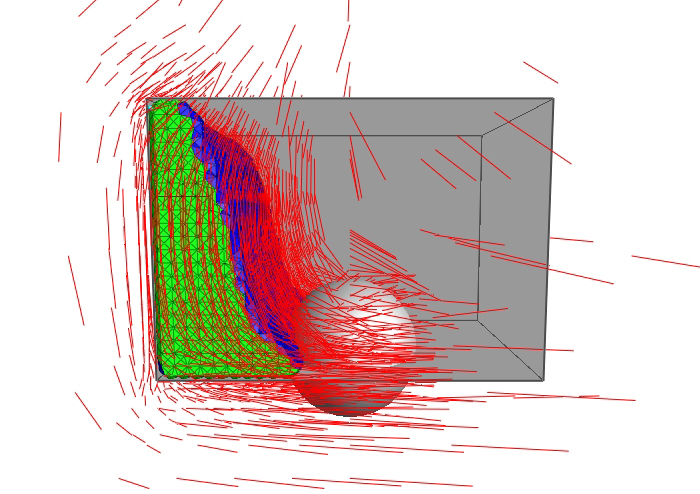
We treat liquid-obstacle (closed) faces using non-slip boundary conditions, or in other words, by matching the face velocity with that of the obstacle (i.e. zero). We follow [FOK05] by setting the pressure outside the mesh (in the obstacle) to be equal to that of the tetrahedron in the mesh. This ensures that the pressure does not change the closed face velocity. Since we are simulating a liquid and not a gas, we must account for the effects of air pressure in the simulation domain. Otherwise, as prior tests have shown, our liquid will behave more like a gas and its velocity field will not be damped, resulting in strange behavior like liquid unrealistically traveling up walls and across ceilings, etc. Therefore for liquid-air (open) faces, we set the pressure outside the mesh to be proportional to the pressure at each tetrahedron in the mesh (around 50-60%). This differs from [FOK05] who set the ambient pressure to 0 to simulate a gas. We place this pressure at a perpendicular distance equal to that of the distance to the pressure in the mesh. |
|
Algebraic Multigrid Solver |
|
Equation
(14) reduces to the system We use the recommendation of [CFLOS07] to solve for the pressure using an algebraic multigrid solver. The authors claim it is twice as fast as traditional preconditioned conjugate gradient solvers. While the details of the solver are in the original paper, this section provides a brief overview. Multigrid
works by computing a quick, inaccurate solution to the system, then
corrects the error with help from an approximate solution to a coarser
version of the problem, which can be solved more quickly. We recursively
solve coarser versions of the problem until the base case is a linear system
small enough to be solved by a direct method. In a geometric
multigrid approach, regular spatial grids of different resolutions guide the
reduction of the system to coarser resolutions. However, the authors
note that this approach is not suitable for tetrahedral meshes on
irregularly shaped domains, as clustering unstructured tetrahedra does not create
larger tetrahedra. In this case it is more appropriate to use an algebraic
multigrid approach that relies solely on the structure of the system matrix
Algebraic multigrid relies on a sequence of linear prolongation matrices that expand a coarse solution to a finer one (via an exact interpolation), and restriction matrices that reduce a fine solution to a coarser one (via an approximate projection). [CFLOS07] provide an algorithm to compute these matrices at each level from the connectivity of adjacent tetrahedra in the system matrix of each level. The authors use 2 Gauss-Seidel iterations to find approximate solutions (usually with poor accuracy) to a given system. Although this may be appropriate for high resolution simulations, using at least 10 iterations is more appropriate for lower resolutions to substantially improve the preservation of fluid volume with minimal computational expense.
Once we have solved for the pressure vector
|
|
|
|
(15) |
|
where
|
|
|
Obstacles |
|
We follow [CFLOS07] to update both the surface contour and mesh to prevent penetration of obstacles. We build a separate signed distance function for the obstacle, using an opposite signing convention to that of the original input function (i.e. if we use positive distances for inside the liquid, we would use negative distances for inside the obstacle). The input to our surface contour and mesh generator is the minimum (or maximum, depending on signing convention) of its original signed distance function and the one for obstacles. Generally, the mesh does not perfectly conform to obstacles and persistent thin gaps can occur between the liquid and obstacles. We fix this after the mesh is built by snapping vertices that are within the distance of one eighth of the mesh generator’s octree edge length to the obstacle, by projecting them orthogonally to the obstacle. It is important to prevent all four vertices of a tetrahedron from snapping to an obstacle (possibly producing a flat tetrahedron of zero volume). |
|
Thickening |
|
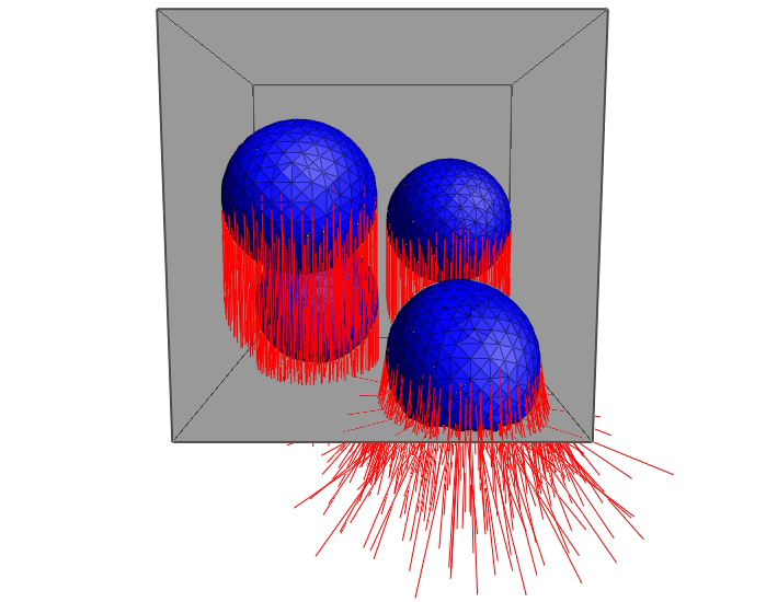
A common problem in liquid simulation is total volume loss over the course of the simulation. This is caused by the numerical errors that accumulate through discrete time steps along the velocity field and the approximation of the surface volume with a tetrahedral mesh. Moreover, thin fluid regions cannot be resolved when they drop below the minimum resolution of the simulation mesh, resulting in rapid volume loss. To address this, we use the novel thickening method of [CFLOS07] to artificially restore volume to the surface contour and mesh. We heuristically detect thin regions of the fluid by shooting a ray backwards from each surface point opposite the surface normal direction and detecting its first intersection point with the surface. If a thin region is detected within a distance threshold, we create thickening particles, shown to the right, near its medial axis which we approximate as the midpoint between the surface point and intersection point. We use the signed distance function at this midpoint to approximate the distance from the axis to the surface, using it as the particle radius. We advect the particles forward using a second-order Runge-Kutta method and make sure to prevent them from penetrating obstacles. These particles are then used to update the input function to both our surface contour and mesh generator. We use the thickening parameters and kernels as recommended by [CFLOS07], despite using a lower resolution simulation where these thickening parameters cause noticeable explosions of volume in the mesh. Ideally, we could have adjusted these parameters to limit the amount of thickening, but in doing so we would have introduced extra volume loss and prevented some thin regions from being simulated, detracting from the overall quality of the fluid flow. |
|

|
Rendering |
|
All animations were rendered in PIXIE, an Open Source renderer that implements the RenderMan interface. As mentioned earlier, at lower mesh resolutions the thickening scheme produces explosions of volume that are unattractive but necessary for good fluid flow. To circumvent this, we render the higher resolution surface contour rather than the tetrahedral mesh that [CFLOS07] render. Rendering the surface contour produces a smoother and more attractive liquid appearance but unfortunately has its disadvantages. For one, folds and creases in the surface contour are visible as two liquid boundaries are in the process of merging. We also lose detail along the liquid surface since the surface contour tends to remain smooth during more turbulent flows. It would have been ideal to avoid these problems by rendering the mesh, if it had been possible to run a higher resolution simulation. |
|
Splashing |
|
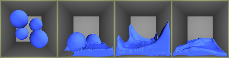
The animations generated by [CFLOS07] depict rich and complex splash patterns that are undoubtedly attributed to their high resolution simulations (using around one million tetrahedra) and their rendering of the tetrahedral mesh as opposed to the surface contour. Preliminary tests have demonstrated that increasing the resolution of the simulation greatly improves liquid splash detail since it supports the simulation of smaller liquid structures that tend to break apart by the thickening scheme. These tests have also shown that increasing the resolution, thereby making the thickening scheme less detectable and allowing us to render the tetrahedral mesh, also captures the splash detail that the surface contour tends to smooth out. Unfortunately, these high resolution tests quickly suffer from unreasonable computation times, despite various optimizations. |
|
Optimizations |
|
A challenging aspect of this project was the necessity to optimize code wherever possible to allow a reasonable resolution during simulation. Decreasing overall simulation time ultimately helped with testing code and parameter modifications that affected the liquid animations. This section describes the main optimizations used in this project. It was imperative to develop a sparse matrix class to improve the performance of the pressure solver and keep memory usage efficient. The best results were obtained by representing both the rows and columns separately as a vector of maps; each map represents one row/column and associates indices within the row/column to corresponding non-zero values. Although the non-zero values are duplicated in this storage scheme, it supports fast entry retrieval/updates within a specific row or column. The most important matrix operation to optimize was multiplication, as the pressure solver uses multiplication to reduce system matrices to coarser resolutions. We can efficiently perform this operation by iterating over all non-zero entries of the left matrix and observe that each of these entries will only be multiplied with the non-zero entries of the corresponding row of the right matrix. We can thereby increment the appropriate element of the product matrix with each of these individual multiplications. The tetrahedral mesher was optimized by reusing vertex, edge, face, and tetrahedron structures wherever possible to minimize memory usage and simplify the connectivity in both the mesh and octree. It was important to limit signed distance function evaluations, a major source of inefficiency in the mesher, by computing these values for only the vertices that required them and only once per vertex. To find the closest vertex to an arbitrary location (for generalized barycentric interpolation), we first find the containing octant in the octree, perform standard walking point location over tetrahedra in the octant to find the containing tetrahedron, and then find the closest vertex in this tetrahedron. During thickening, we can improve the performance of detecting ray-surface intersections by collecting surface triangles within a distance threshold from the ray (using the octree) and only perform ray-triangle intersections on them. Lastly, due to the lengthy time required to generate animations (lasting up to 12 hours!), it was necessary to add the ability to save and restore simulation states to recover from problems during simulation. |
|
Results |
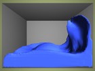
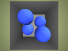
 (click to watch movie) 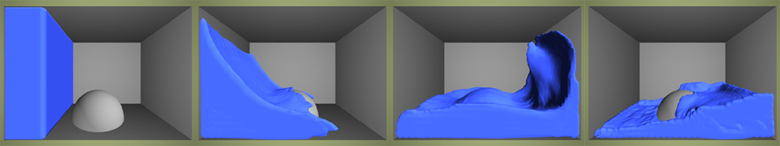 (click to watch movie) 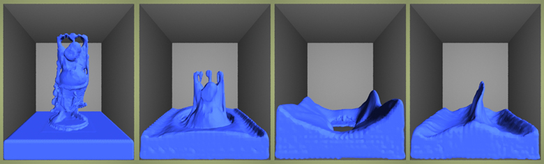 (click to watch movie) |
|
All three of the above liquid animations were generated on a Sony Vaio laptop with a 2.0 GHz Intel Core 2 Duo processor (T7200) and 2 GB of memory. The tetrahedral mesh generator’s octree contained 6 levels of octants (with 7 levels for the surface contour) producing meshes that contained an average of 10-20K tetrahedra. Each animation was roughly 300-400 frames in length at 60 frames per second, with each frame requiring 30 seconds to 2 minutes of computation time to generate. |